Sea-Level Report Cards
Chesapeake Bay
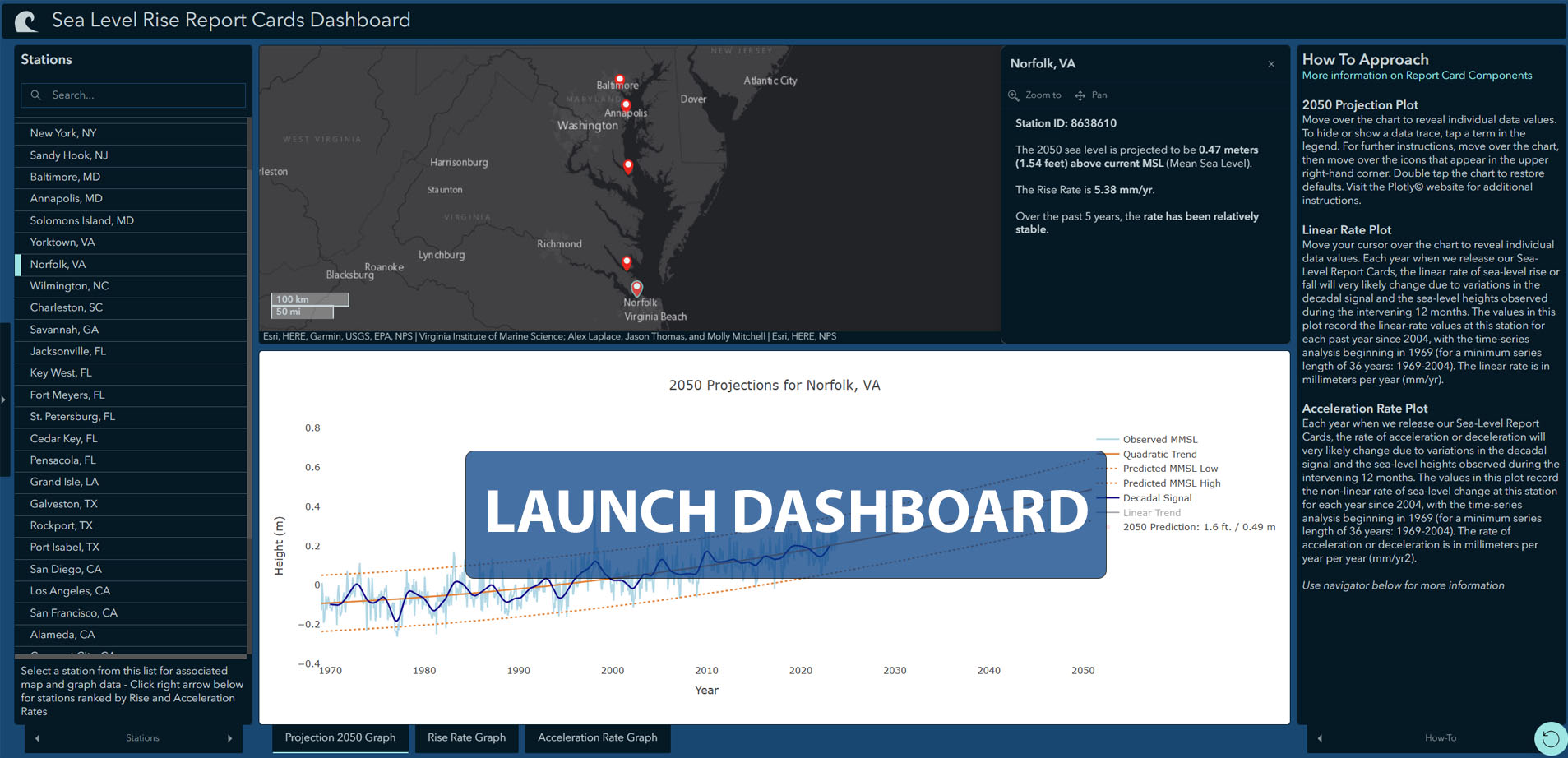
Want to know how sea level in the Chesapeake Bay is changing due to global warming and other factors? Our 'report cards' can help. Updated by the Virginia Institute of Marine Science each year as annual tide-gauge data become available, they display recent sea-level trends and project sea-level height to the year 2050 for localities along the U.S. East, Gulf, and West coasts, including 5 localities from north to south within the Chesapeake Bay.
Sea-level projections vary from place to place along the Bay shoreline due to local differences in the processes that control sea-level rise, particularly land subsidence. Launch the dashboard below to compare projections for Norfolk and Yorktown, Virginia with those for Annapolis, Baltimore, and Solomons Island, Maryland.
To learn how to interact with and read the projection charts, expand the selections below.
How to Interact with your Projection ChartMove over the chart to reveal individual data values. To hide or show a data trace, tap a term in the legend. For further instructions, move over the chart, then move over the icons that appear in the upper right-hand corner. Double tap the chart to restore defaults. Visit the Plotly© website for additional instructions. |
Observed MMSLRepresented in light blue, the Monthly Mean Sea Level (MMSL) shows the height of the water at this tidal gauge averaged over a calendar month of measurements corrected by removing predictable tidal variations. Thus the sharp ups and downs reflect almost entirely non-tidal changes in water level due to storms and shifts in ocean and estuarine circulation. Height is measured relative to a standard elevation defined by the National Oceanic and Atmospheric Administration. (NOAA) We obtain the raw monthly mean sea-level measurements for our report cards from NOAA's official tidal station network. We do so because these measurements represent the value we are most concerned with—the rate of sea-level change relative to piers, buildings, homes, and streets. These measurements of "relative mean sea level" (RMSL) account not only for global changes in the volume of sea water—driven by factors such as thermal expansion of the ocean and melting of ice sheets, but also local movements of the land as shorelines rise, sink, or remain stable in response to groundwater removal, glacial isostatic adjustment, and other factors. We obtain the RMSL data from the NOAA/National Ocean Service at www.tidesandcurrents.noaa.gov. The site offers its users a choice of tidal datums—a base elevation used as a reference from which to reckon the tidal height. We use mean sea level (MSL), a reference defined at U.S. primary tide stations as the average water level over a series of years (currently 1983-2001). The MSL datum approximates where sea level stood mid-series in the year 1992. Sea-level values are negative if below the height of mean sea level during this year. |
Quadratic TrendThe quadratic trend, shown in darker orange, indicates that sea level is not only rising at this tidal station, but that the rate of sea-level rise is accelerating with time. In other words, the rate of sea-level rise is best represented by a quadratic curve rather than a straight line. Comparing the quadratic and linear projections shows an exponential rise in sea level will result in a significantly higher sea level in future yearsIf the best fit to a series of monthly mean sea-level data is a non-linear trend, it implies that sea level has either accelerated or decelerated during the given period. If acceleration or deceleration is assumed constant, then the curve fitted is described by a quadratic equation. A conventional analysis fitting a quadratic curve yields two coefficients, symbolized here by β1 and β2. β1 represents sea-level rise (or fall if negative) in millimeters per year (mm/year), whereas β2 represents acceleration (deceleration if negative) in mm/year2. For each report card, we have analyzed the quadratic trend to determine whether either coefficient is statistically significant (different from zero). The precaution about a linear trend (β1) not remaining constant with time is doubly important in the case of a non-linear trend where acceleration (β2) is likely to be much more variable. Where a pattern of non-linear change can be seen it is well worth noting because, if it persists, a very different outcome could result compared to that derived from a strictly linear projection of sea level forward in time. For further details, read Evidence of Sea Level Acceleration at U.S. and Canadian Tide Stations, Atlantic Coast, North America (Boon 2012). |
QHi95 and QLo95Shown in dotted orange, these confidence intervals encompass 95% of the sea-level observations recorded during each month at this tidal station, whether above (QHi95) or below (QLo95) the mean. Extending these intervals forward implies that sea level could be of equal magnitude higher or lower than the best (quadratic) estimate of sea level during any future month out to 2050. |
Linear TrendThe linear trend, shown in green, indicates how quickly sea level would rise at this tidal station with no acceleration in the rise rate (our analysis suggests this is not the case). We display the linear trend to help clarify that linear projections result in a significantly lower sea level in future years than we expect given recent observations of an accelerating rate of sea-level rise at this station.Public projections of sea-level change most commonly use a linear trend—a straight line fitted to a time-series plot of monthly (or annual) mean sea level heights. The trend is the slope of the line expressed (usually) in millimeters per year (mm/yr). A positive slope, if statistically different from zero, implies a constant rise in sea level at the rate shown for the period given; a significant negative slope implies that sea level is falling at a constant rate for the given period. Whereas use of a linear trend may be an appropriate approach for concerns about sea-level rise in the near term and for regional, national, and global scales, it has several drawbacks:
For these and other reasons, we have chosen to base our sea-level projections on non-linear, exponential trends as explained in the following section. We display the linear trend in our sea-level report cards to help clarify that linear projections result in a significantly lower sea level in future years than we expect given recent observations of an accelerating rate of sea-level rise at many tidal stations. |
Decadal SignalThe decadal signal, shown in dark blue, portrays ups and downs in sea level due to relatively short-term interactions between the oceans and the atmosphere, with El Niño as an example. Projections to 2050 made during an upturn in the decadal signal will be higher than they would be if the decadal signal was nearing or at a low. Learn more about the long- and short-term processes that influence sea level. |
Why 2050?
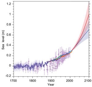
Predicting water levels as far forward as 2100—an appropriate horizon for the global considerations addressed by the IPCC—requires the use of physics-based models, as sea-level observations alone cannot be "extrapolated" to the end of the century with any certainty. However, if we choose a closer target—the year 2050—we find there is sufficient historical data to allow inferences based on observed trends. This is the approach that we have adopted in our sea-level report cards. The year 2050 is also an appropriate time frame for use in planning by citizens, property owners, and municipalities. |
Why 1969?Most of the tide-gauge stations that provide the data used in our sea-level report cards began operation in the first few decades of the 1900s or even earlier. However, many stations—particularly along the U.S. East Coast—show evidence of a non-linear change or acceleration beginning in 1987, at the center of a 36-year sliding window beginning in 1969—thus setting the start date for our sea-level report cards. In short, we use post-1969 data because the linear sea-level trends of earlier decades do not accurately predict the sea-level changes that are most likely to occur given more recently observed acceleration in the rate of sea-level rise. |
Year-to-Year Trends
How to Interact with your Trend ChartsMove your cursor over the chart to reveal individual data values. To move between the two charts, tap an index tab. |
Annual Linear RateEach year when we release our Sea-Level Report Cards, the linear rate of sea-level rise or fall will very likely change due to variations in the decadal signal and the sea-level heights observed during the intervening 12 months. The values in this plot record the linear-rate values at this station for each past year since 2004, with the time-series analysis beginning in 1969 (for a minimum series length of 36 years: 1969-2004). The linear rate is in millimeters per year (mm/yr). |
Annual Acceleration RateEach year when we release our Sea-Level Report Cards, the rate of acceleration or deceleration will very likely change due to variations in the decadal signal and the sea-level heights observed during the intervening 12 months. The values in this plot record the non-linear rate of sea-level change at this station for each year since 2004, with the time-series analysis beginning in 1969 (for a minimum series length of 36 years: 1969-2004). The rate of acceleration or deceleration is in millimeters per year per year (mm/yr2). |
Processes
LegendOur Processes page provides a comprehensive explanation of the processes that affect sea level on global, regional, and local scales. |
Steric ProcessesSteric processes describe changes in the density and volume of seawater due to changes in its temperature (thermosteric) or salinity (halosteric). Warming and freshening reduces the density of seawater, thus increasing its volume and contributing to sea-level rise. Cooler and saltier water is more dense, occupies less volume, and thus contributes to sea-level fall. Steric processes are important to global predictions of climate-mediated sea-level change such as those issued by the IPCC. |
Glacial Isostatic Adjustment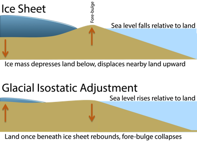 GIA is the response of the Earth’s surface to the unloading of ice-sheet and glacial mass. This results in upward motion (rebound) of the land surface in areas previously covered by ice, and subsidence (fore-bulge collapse) in land areas previously displaced upward by the adjacent ice-sheet “dimple.” Subsidence of a coastal area equates to a rise in sea level relative to the land, and vice versa. GIA is the response of the Earth’s surface to the unloading of ice-sheet and glacial mass. This results in upward motion (rebound) of the land surface in areas previously covered by ice, and subsidence (fore-bulge collapse) in land areas previously displaced upward by the adjacent ice-sheet “dimple.” Subsidence of a coastal area equates to a rise in sea level relative to the land, and vice versa. |
Water or Oil Withdrawal/StorageWithdrawal of groundwater or hydrocarbons such as oil and gas can lead to a relative rise in sea level due to local subsidence of the land surface. These localized processes are likely to affect only one or two tide stations and therefore contribute greatly to regional variation. Understanding their magnitude and impact is critical for adaptation and management efforts, since pumping can be controlled relatively easily. Past subsidence can also greatly impact sea-level trends and thus must be carefully considered when choosing the appropriate length of record to analyze. |
Eustatic Processes (Glacial Melt, etc.)Eustatic processes describe changes in the mass of water in the oceans. Melting of ice sheets and glaciers; increased runoff from lakes, rivers, and groundwater; and increased oceanic precipitation all lead to eustatic sea-level rise. These processes are important to global predictions of climate-mediated sea-level rise such as those issued by the IPCC. |
Ocean Dynamics
|
Atmospheric ProcessesThe “inverted barometer” effect is the response of ocean height to atmospheric pressure. Sea level rises beneath a low-pressure system, most noticeably during hurricanes and other intense storms. Conversely, sea level falls beneath a high-pressure cell, as seen during periods of clear, calm weather. Consistent winds can produce a similar effect, pushing water levels higher downwind and causing water levels to fall upwind. Although pressure and wind effects act in the short term, they may affect the trends seen in long-term tide-gauge analyses and thus need to be considered in our analysis. |
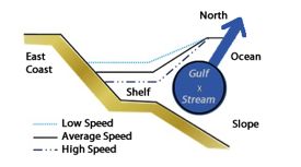 Shifts in ocean currents and water masses can affect sea-level height; for instance, a weakening of the Gulf Stream (as predicted by climate-change models) can
 Station Facts
| Locality | NOAA Station ID | Station Established |
| Baltimore, MD | 8574680 | Jul 01, 1902 |
| Annapolis, MD | 8575512 | Sep 14, 1978 |
| Solomons Island, MD | 8577330 | Nov 05, 1937 |
| Yorktown, VA | 8637689 | Jan 22, 2004* |
| Sewells Point, VA | 8638610 | Jul 01, 1927 |