2010 SAV Report

Organizational Procedures

Black-and-white aerial photography at a scale of 1:24,000 was the principal source of information used to assess distribution and abundance of SAV in Chesapeake Bay, its tributaries, and the Delmarva Peninsula coastal bays from Assawoman Bay to Magothy Bay in 2010. There were 175 flight lines that yielded aerial photography negatives that were scanned and orthorectified to create orthophoto mosaics. These mosaics were carefully examined on-screen and outlines were drawn to identify all SAV beds visible on the photography, providing a geographic information system (GIS) digital database for analysis of bed areas and locations. Ground survey information collected in 2010 was tabulated and entered into the VIMS SAV GIS digital database.

The aerial photography is carefully examined to identify all visible SAV beds. Photographs covering SAV beds are scanned and orthorectified to create orthophoto mosaics. Outlines of SAV beds are then interpreted on-screen, providing a digital database for analysis of bed areas and locations. Ground survey information collected in 2010 is tabulated and entered into the SAV geographic information system (GIS). SAV distribution data are presented and discussed based on the 2003 revised Chesapeake Bay Program (CBP) segmentation and zonation scheme (DAWG, 1997). This segmentation scheme is mapped, listed by salinity regime, and delineated descriptively.

The CBP Segmentation scheme defines 93 segments that are grouped into three zones for this report. The Upper Bay Zone includes the Susquehanna River and extends to the Chesapeake Bay Bridge; the Middle Bay Zone extends to the southern boundaries of CB5MH, TANMH, and POCMH; the Lower Bay Zone extends to the mouth of Chesapeake Bay and includes the James River. The salinity within each zone roughly coincides with the major salinity zones of estuaries:

• Oligohaline Upper Zone (0.5-5 ppt)
• Mesohaline Middle Zone (5-18 ppt)
• Polyhaline Lower Zone (18-25 ppt)

SAV Species

The term "submerged aquatic vegetation" (SAV) for the purpose of this report encompasses twenty-three taxa from twelve vascular macrophyte families and three taxa from one freshwater macrophytic algal family, the Characeae. The term "SAV" in this report excludes all other algae, both benthic and planktonic, which occur in Chesapeake Bay, its tributaries, and the Delmarva Peninsula coastal bays. Although these other algae species constitute a portion of the SAV biomass in this region (Humm, 1979), this survey did not attempt to identify, delineate, or discuss the algal component of the vegetation nor its relative importance in the flora. The aerial survey cannot differentiate epiphytic algae on submersed vascular plants or differentiate many benthic marine algae species, including many macrophytes, which can co-occur in the same SAV beds.

Seventeen species of submerged aquatic vegetation are commonly found in Chesapeake Bay and its tributaries. Zostera marina (eelgrass), the only "true" seagrass species, can tolerate salinities as low as 10 ppt and is dominant in the lower reaches of the bay. Myriophyllum spicatum (Eurasian watermilfoil), Stuckenia pectinata (sago pondweed), Potamogeton perfoliatus (redhead grass), Potamogeton crispus (Curly pondweed), Potamogeton pusillus (Slender pondweed), Zannichellia palustris (horned pondweed), Vallisneria americana (wild celery), Elodea canadensis (common elodea), Ceratophyllum demersum (coontail), Hydrilla verticillata (hydrilla), Heteranthera dubia (water stargrass), Najas guadalupensis (southern naiad), Najas minor, Najas gracillima, and Najas sp. are freshwater species, some of which have the capacity to tolerate some level of salt, and are found in the middle and upper reaches of the bay (Stevenson and Confer, 1978; Orth et al., 1979; Orth and Moore, 1981, 1983; Moore et al., 2000). Ruppia maritima (widgeon grass) is tolerant of a wide range of salinities and is found from the bay mouth to the Susquehanna Flats. Approximately nine other species are only occasionally found. When present, these less common species occur primarily in the middle and upper reaches of the bay and the tidal rivers. Of all species of SAV, the most abundant are Z. marina, R. maritima, V. americana, H. verticillata, P. perfoliatus, Stuckenia pectinata (P. pectinatus), and M. spicatum.

Zostera marina and R. maritima are the dominant SAV species found in the Delmarva Peninsula coastal bays.

An online key to Chesapeake Bay SAV is available from the Maryland Department of Natural Resources web page.

Aerial Photography

The 2014 aerial multispectral digital imagery was obtained by Air Photographics (Martinsburg, West Virginia) using a Wild RC-30 camera, with a 153 mm (6 inch) focal length Aviogon lens and Agfa Pan 80 film, mounted in the bottom fuselage of a Piper Aztec, a twin engine reconnaissance aircraft. Photography was acquired from an altitude of approximately 12,000 feet, yielding 1:24,000 scale photographs. A Novatel DL dual frequency GPS and an Applanix Phalanx IMU was attached to the camera to acquire IMU data.

The 197 flight lines, which cover 4,335 flight line kilometers, were numbered and included land features necessary to establish control points for accurate mapping if IMU data was not available. The flight lines used to obtain the photography were positioned to include all areas known to have SAV, as well as most areas that could potentially have SAV in the Middle and Upper zones (i.e., all areas where water depths were less than two meters at mean low water).

Flight lines were prioritized by sections and flights were timed during the peak growing season of species known to inhabit each area. In addition, specific areas with significant SAV coverage were given priority.

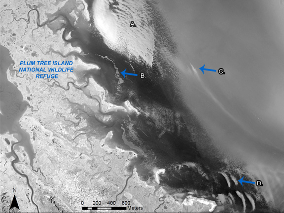
Guidelines for acquisition of aerial photography address tidal stage, plant growth, sun angle, atmospheric transparency, turbidity, wind, sensor operation, and land features. Adherence to the guidelines assured acquisition of photography under nearly optimal conditions for detection of SAV, thus ensuring accurate photo interpretation. Deviation from any of these guidelines required prior approval by VIMS staff. Quality assurance and calibration procedures were consistently followed. The altimeter was calibrated annually by the Federal Aviation Administration and the aerial camera was calibrated by USGS.

Camera settings were selected by automatic exposure control. Sun angle was measured with a sensor on the plane. Flight lines were plotted on 1:250,000 scale maps to allow for overlap of photography. To minimize image degradation due to sun glint, the camera was equipped with a computer controlled intervalometer which established 60% line overlap and 20% sidelap. An automatic bubble level held the camera to within one-degree tilt. The scale, altitude, film, and focal length combination was coordinated so that SAV patches of one square meter could be resolved. Ground-level wind speed was monitored hourly. Under normal operating conditions, flights were usually conducted under wind speeds less than 10 mph. Above this speed, wind-generated waves stir bottom sediments, which can easily obscure SAV beds in less than one hour. The pilot used experiential knowledge to determine the acceptable level of turbidity that would allow complete delineation of SAV beds. During optimum flight conditions the pilot was able to distinguish bottom features such as SAV or algae at low tide. Excessively turbid conditions precluded photography. Determination of optimum cloud cover level was based on pilot experience. Records of this parameter were kept in a flight notebook. Every attempt was made to acquire photographs when there was no cloud cover below 12,000 feet. Cloud cover did not exceed 5% of the area covered by the camera frame. A thin haze layer above 12,000 feet was generally acceptable. Experience with the Chesapeake Bay has shown that optimal atmospheric conditions generally occur two to three days following passage of a cold front, when winds have shifted from north-northwest to south and have moderated to less than 10 mph. Within the guidelines for prioritizing and executing the photography, the flights were planned to coincide with these atmospheric conditions when possible. Air Photographics coordinated the processing of all film. A 9-inch by 9-inch, black-and-white contact print was produced for each exposed frame. Each photograph was labeled with the date of acquisition as well as the flight line number. Film and photographs are stored under appropriate environmental conditions to prevent degradation.

Mapping Process

Black-and-white aerial photography at a scale of 1:24,000 is carefully examined to identify all visible SAV beds. Aerial photography negatives covering SAV beds are scanned and orthorectified to create orthophoto mosaics. Outlines of SAV beds are then interpreted on-screen, providing a digital database for analysis of bed areas and locations. Ground survey information collected in 2010 is tabulated and entered into the SAV geographic information system (GIS).

USGS 7.5 minute quadrangle maps are used to organize the mapping process, including interpretation of SAV beds from aerial photography, mapping ground survey data, and compiling SAV bed area measurements. The SAV quadrangle index page gives locations of the 258 quadrangles in the study area that includes all regions with potential for SAV growth. Most quadrangles are sequentially numbered for efficient access to data.

Orthorectification and Mosaic Production
Scanned aerial photography negatives are georectified and orthographically corrected to produce a seamless series of aerial mosaics following the standard operating procedures (SOP). ERDAS IMAGINE Leica Photogrammetry Suite (LPS) image processing software is used to orthographically correct the individual flight lines using a bundle block solution. Camera lens calibration data is matched to the image location of fiducial points to define the interior camera model. Control points from USGS DOQQ images provide the exterior control, which is enhanced by a large number of image-matching tie points produced automatically by the software. The exterior and interior models are combined with a 30-meter resolution digital elevation model (DEM) from the USGS National Elevation Dataset (NED) to produce an orthophoto for each aerial photograph.

The orthophotographs that cover each USGS 7.5 minute quadrangle area are adjusted to approximately uniform brightness and contrast and are mosaicked together using the ERDAS Imagine mosaic tool, producing a one-meter resolution quad-sized mosaic.

Photo Interpretation and Bed Delineation
The SAV beds are interpreted on-screen from the orthophoto mosaics using ESRI ArcInfo GIS software. The identification and delineation of SAV beds by photo interpretation utilizes all available information including: knowledge of aquatic grass signatures on film, distribution of SAV in 2010 from aerial photography, 2010 ground survey information, and aerial site surveys.

In addition to delineating SAV bed boundaries, an estimate of SAV density within each bed was made by visually comparing each bed to an enlarged crown density scale similar to those developed for estimating crown cover of forest trees from aerial photography (Paine, 1981). Bed density was categorized into one of four classes based on a subjective comparison with the density scale. These were: 1, very sparse (<10% coverage); 2, sparse (10-40%); 3, moderate (40-70%); or 4, dense (70-100%). Either the entire bed or subsections within the bed were assigned a bed density number (1 to 4) corresponding to the above density classes. Some beds were subsectioned to delineate variations of SAV density. Additionally, each distinct SAV bed or bed subsection was assigned an identifying one or two letter designation unique to its map. Coupled with the appropriate SAV quadrangle number and year of photography, these letter designations uniquely identify each SAV bed in the database.

Standard operating procedures (SOPs) were developed to facilitate orderly and efficient processing of 2010 SAV maps and SAV computer files produced from them, and to comply with the need for consistency, quality assurance, and quality control. SOPs included: a detailed procedure for orthorectification, mosaicking, and photo-interpretation; tracking sheets to record the processing of flight lines and quadrangles; and weekly summary progress reports of all operations.

Calculation of Area

An ArcGIS geodatabase in a Universal Transverse Mercator (UTM) Zone 18 projection was used to calculate area in square meters for all SAV beds. These areas are summarized by USGS 7.5 minute quadrangle, Chesapeake Bay Program and Delmarva Peninsula coastal bay segments, and by zone in tables. Segment and zone totals were calculated using an overlay operation of segment and zone regions on the SAV beds.

Ground Surveys

Ground surveys were accomplished by cooperative efforts from a number of agencies and individuals. Although not all areas of Chesapeake Bay were ground surveyed, the data did provide valuable supplemental information. The ground surveys confirmed the existence of some SAV beds mapped from the 2010 1:24,000 scale aerial photography, as well as SAV beds that were too small to be visible on the 1:24,000 scale photography. The surveys also provided species data for many of the SAV beds. Ground survey information supplied to VIMS researchers is included on the SAV distribution and abundance digital maps and included in the VIMS SAV GIS Database. The group that performed each survey is designated by a unique symbol to identify the different methods of sampling. In many cases the symbols on the SAV maps have been offset from the actual sampling point to avoid confusion with the mapped SAV bed. Where species information was available, it is included on the map. Because of space limitations on the maps, occasionally one or more survey points are combined where the information was duplicated. All ground survey data supplied to VIMS are tabulated in the ground survey table.

Ground survey data were obtained in 2010 by:

• Peter Bergstrom of National Oceanic and Atmospheric Administration (NOAA) for Jug Bay; Magothy, Severn, Back, Bush, Patapsco, and Choptank rivers; and Susquehanna Flats
• Jessica Alexander, and Lauren Leese of Maryland Environmental Service (MES) for Hart-Miller Island
• Candace Croswell of Baltimore County Department of Environmental Protection and Resource Management (BCDEPRM) for Middle, Gunpowder, Back, Patapsco, and Bird rivers
• Patricia Delgado, Rebecca Golden, Lee Karrh, and Mark Lewandowski of Maryland Department of Natural Resources (MD-DNR) for Bush, Choptank, Elk, Gunpowder, Honga, Patuxent, Potomac, Sassafras, and Severn rivers; Isle of Wight and Jug bays; and Susquehanna Flats
• Roman Jesien of Maryland Coastal Bays Program (MCBP) for Isle of Wight Bay
• Daniel Ryan of District of Columbia Fisheries and Wildlife Division (DCFWD) for Potomac River
• Brian Sturgis of National Park Service (NPS) for Sinepuxent and Chincoteague bays
• Terry Willis of Chesapeake College (CC) for Chester River
• Chris Guy of United States Fish and Wildlife Service (USFWS) for Eastern Bay
• Evamaria Koch and Becky Swerida of University of Maryland Center for Environmental Science - Horn Point Laboratory (UMCES) for Tangier Sound; and Severn, Choptank, Patuxent, and Honga rivers
• Virginia Institute of Marine Science (VIMS) for areas of the Chesapeake that include Mattaponi, Pamunkey, Chickahominy, Piankatank; York, Back, and James rivers; Broad and Mobjack bays; Tangier and Pocomoke sounds; and Magothy, South, and Cobb bays along the eastern shore of the Delmarva Peninsula

Literature Cited

• DAWG. 1997. Chesapeake Bay Program Analytical Segmentation Scheme for the 1997 Re-evaluation and Beyond. Chesapeake Bay Program (CBP) Monitoring Subcommittee (MSC) Data Analysis Work Group (DAWG). Draft December 15, 1997 (amended and approved January 29, 1998).
• Godfrey, R. K. and J. W. Wooten. 1979. Aquatic and Wetland Plants of Southeastern United States: Monocotyledons. The University of Georgia Press, Athens, GA. 712 pp.
• Godfrey, R. K. and J. W. Wooten. 1981. Aquatic and Wetland Plants of Southeastern United States: Dicotyledons. The University of Georgia Press, Athens, GA. 933 pp.
• Harvill, A. M., C. E. Stevens, and D. M. E. Ware. 1977. Atlas of the Virginia Flora: Part I, Pteridophytes through Monocotyledons. Virginia Botanical Associates, Farmville, VA. 59 pp.
• Harvill, A. M., T. R. Bradley, and C. E. Stevens. 1981. Atlas of the Virginia Flora: Part II, Dicotyledons. Virginia Botanical Associates, Farmville, VA. 148 pp.
• Humm, Harold J. 1979. The Marine Algae of Virginia. Special Papers in Marine Science, Number 3, Virginia Institute of Marine Science. The University Press of Virginia, Charlottesville, VA. 263 pp.
• Kartesz, J. T. and R. Kartesz. 1980. A Synonymized Checklist of the Vascular Flora of the United States, Canada and Greenland: Volume II, The Biota of North America. The University of North Carolina Press, Chapel Hill, NC. 498 pp.
• Moore, K. A., D. J. Wilcox, and R. J. Orth. 2000. Analysis of the Abundance of Submersed Aquatic Vegetation Communities in the Chesapeake Bay. Estuaries. 23:115-127.
• Orth, R. J., K. A. Moore, and H. H. Gordon. 1979. Distribution and Abundance of Submerged Aquatic Vegetation in the Lower Chesapeake Bay, Virginia. Final Report to U.S. EPA, Chesapeake Bay Program, Annapolis, MD. EPA-600/8-79-029/SAV1. 38 pp.
• Orth, R. J. and K. A. Moore. 1981. Submerged Aquatic Vegetation in the Chesapeake Bay: Past, Present and Future. pp. 271-283. In: Proc. 46th North American Wildlife and Natural Resources Conf., Wildlife Management Institute, Washington, D.C.
• Orth, R. J. and K. A. Moore. 1983. Chesapeake Bay: An Unprecedented Decline in Submerged Aquatic Vegetation. Science. 222:51-53.
• Paine, David P. 1981. Aerial Photography and Image Interpretation for Resource Management. John Wiley & Sons, Inc., New York City, NY. 571 pp.
• Radford, A. E., H. E. Ahles, and C. R. Bell. 1968. Manual of the Vascular Flora of the Carolinas. The University of North Carolina Press, Chapel Hill, North Carolina, NC. 1183 pp.
• Stevenson, J. C. and N. Confer. 1978. Summary of Available Information on Chesapeake Bay Submerged Vegetation. U.S. Dept. of Interior, Fish and Wildlife Service. FWS/0BS-78/66. 335 pp.
• U.S. Environmental Protection Agency, Region III, Chesapeake Bay Program Office, Annapolis, Maryland and Region III, Water Protection Division, Philadelphia, Pennsylvania, in coordination with Office of Water, Office of Science and Technology, Washington, D.C. Technical Support Document for Identification of Chesapeake Bay Designated Uses and Attainability. 2004 Addendum. October 2004.
• Wood, R. D. and K. Imarhori. 1964. A Revision of the Characeae: Volume II, Iconograph of the Characeae. Verlag Von J. Cramer, Weinheim, Germany. 395 icones with index.
• Wood, R. D. and K. Imahori. 1965. A Revision of the Characeae: Volume I, Monograph of the Characeae. Verlag Von J. Cramer, Weinheim, Germany. 904 pp.

Lists and Figures

Lists

SAV species found in Chesapeake Bay
Guidelines followed during acquisition of aerial photographs
Chesapeake Bay Program and Delmarva Peninsula coastal bay segments with salinity regime
Chesapeake Bay Program and Delmarva Peninsula coastal bay segment descriptions

Figures

Location of 2010 SAV beds in Chesapeake Bay
Index of flight lines for 2010 SAV photography
Index of quadrangles for Chesapeake Bay and the Delmarva Peninsula coastal bays
Index of Chesapeake Bay Program Segments
Segment Comparision Map of Chesapeake Bay and its tributaries
Crown density scale used for estimating density of SAV beds from aerial photography